scFlow - Single-cell/nuclei RNA-seq analysis tools in R for a complete workflow
This vignette was created by Nurun Fancy and Combiz Khozoie
18 February, 2024
Source:vignettes/scFlow.Rmd
scFlow.RmdOverview
The goal of scFlow is to provide tools in R to build a complete analysis workflow for single-cell/nuclei RNA sequencing data.
Quality control of gene-cell matrices
Filtering of matrices by counts and features
Filtering of mitochondrial genes and mitochondrial counts thresholding
Doublet and multiplet identification and removal with DoubletFinder
Rich QC metrics annotation with scater
Dataset integration with Liger
Dimensionality reduction and celltype identification
Louvain clustering, UMAP dimensionality reduction, and cluster marker gene identification with monocle3
Celltype annotation with EWCE
Cluster identity mapping against the Allen Human Brain Atlas
Differential gene expression implementations
Zero-inflated regression model with MAST
Random effects model with Limma
Pathway and functional category enrichment analysis
Interface to the Enrichr database with EnrichR
Interface to the WebGestalt tool with WebGestaltR
Publication quality plots and analysis reports
QC plots and tabular metrics suitable for reports.
UMAP plots for cell features and gene expression.
Violin plots for gene expression.
Pathway and gene enrichment plots
The package functions are designed to interface neatly with NextFlow for scalable and containerized pipelines deployed locally, on high-performance computing clusters, or in the cloud. An accompanying NextFlow pipeline is in the works - TBA.
Install the scFlow and dataset repository
First, install a few dependencies that aren’t automatically installed:
options(repos = "https://cran.r-project.org/", pkgType = "source")
install.packages("Matrix")
install.packages("irlba")
install.packages("Seurat")
install.packages("SeuratObject")
install.packages("lme4")
install.packages("apcluster")
remotes::install_github("NathanSkene/EWCE")
remotes::install_github("chris-mcginnis-ucsf/DoubletFinder")
Now, install the latest version of scFlow.
remotes::install_github("neurogenomics/scFlow")For a detailed explanation on how scFlowExamples dataset was generated, visit this link.
Running scFlow
The scFlow pipeline requires three main input: a folder containing matrix.mtx.gz, features.tsv.gz, barcodes.tsv.gz for individual samples, a SampleSheet.tsv file which is a tab-separated-variable file with sample metadata and a Manifest.txt file is a tab-separated-variable file with two columns: key and filepath. Details of how to generate the files is given in this page
The basic scFlow workflow for sample QC begins with the import of the feature-barcode sparse matrix with read_sparse_matrix. The metadata for the sample is then imported from a sample sheet with read_metadata. A SingleCellExperiment object is created from the matrix and the metadata using generate_sce which is then annotated with both gene and cell-level data using annotate_sce. We then filter the SingleCellExperiment to select only cells and genes meeting our QC criteria using filter_sce. We can then optionally find singlets in our filtered SingleCellExperiment using find_singlets before filtering them out again with filter_sce. A complete QC report can then be generated using report_qc_sce before saving the filtered and quality-controlled SingleCellExperiment with write_sce.
Step one - set up example data & import the matrix and metadata
Call required packages for vignette:
#vignette packages
library(apcluster) #need to load before scFlow to avoid function clash
library(scFlow)
library(SingleCellExperiment)
library(dplyr)
First we must get and format the data from scFlowExamples for the vignette:
#create temp directory to store data
outputDir <- tempdir()

#stored inside tmp_Zeisel2015_scflow inside directory:
destpath <- file.path(outputDir, "tmp_Zeisel2015_scflow.zip")
download.file(url = "https://github.com/neurogenomics/scFlow/releases/download/0.7.2/tmp_Zeisel2015_scflow.zip", destfile = destpath)
unzip(destpath, exdir = outputDir)
unlink(destpath)
list.files(file.path(outputDir,"tmp_Zeisel2015_scflow"))
## [1] "individual_1"    "individual_2"    "individual_3"    "individual_4"
## [5] "individual_5"    "individual_6"    "Manifest.txt"    "SampleSheet.tsv"
Now we can create file paths to each:
#get locations to necessary files
matrix_fp <- file.path(outputDir,"tmp_Zeisel2015_scflow","individual_1")
samplesheet_fp <- file.path(outputDir,"tmp_Zeisel2015_scflow","SampleSheet.tsv")
manifest_fp <- file.path(outputDir,"tmp_Zeisel2015_scflow","Manifest.txt")
#Also need mapping and ctd file which can be downloaded
ensembl_fp <- file.path(outputDir, "ensembl_mappings.tsv")
download.file(url = "https://github.com/neurogenomics/scFlow/releases/download/0.7.2/ensembl_mappings_human.tsv", destfile = ensembl_fp)

ctd_fp <- file.path(outputDir, "ctd_folder")
dir.create(ctd_fp)
download.file(url = "https://github.com/neurogenomics/scFlow/releases/download/0.7.2/ctd_AIBS_v2.rds", destfile = file.path(ctd_fp, "ctd_AIBS_v2.rds"))
To run scFlow, we first need to read in the data matrix:
mat <- read_sparse_matrix(matrix_fp)Next, we retrieve the metadata by pointing to a Sample Sheet and specifying a unique identifier (unique_key) in a specific column (key_colname):
#get name generated for first row in case changes
first_sample <- read.table(file = samplesheet_fp,
                           sep = '\t', header = TRUE)[1,1]
metadata <- read_metadata(
  unique_key = first_sample,
  key_colname = "manifest",
  samplesheet_path = samplesheet_fp
)
##
## ── Reading sample metadata ─────────────────────────────────────────────────────
## Reading /tmp/RtmpWmQoYJ/tmp_Zeisel2015_scflow/SampleSheet.tsv
##
## ✔ Five metadata variables loaded for manifest='majos'
## manifest: `majos` (factor)
## individual: `1` (integer)
## diagnosis: `Cases` (factor)
## sex: `F` (factor)
## age: `15` (integer)
For downstream analyses it’s important that the variable classes are correctly specified. Carefully inspect the metadata classes in brackets. In the above example we see that the individual were imported as integer rather than factor variables. Let’s correct this by reloading the metadata, this time specifying the correct variable classes for this variable:-
var_classes <- c(
  individual = "factor"
)

metadata <- read_metadata(
  unique_key = first_sample,
  key_colname = "manifest",
  samplesheet_path = samplesheet_fp,
  col_classes = var_classes
)
## Reading /tmp/RtmpWmQoYJ/tmp_Zeisel2015_scflow/SampleSheet.tsv
##
With the metadata imported with the correct variable classes, and the previously loaded sparse matrix, we can generate our SingleCellExperiment object:-
sce <- generate_sce(mat, metadata)The SingleCellExperiment object was succesfully created and we can now proceed with annotation.
Step two – Modelling ambient RNA profiling and annotating the SingleCellExperiment
For snRNAseq data generated by 10X genomics, the initial mapping of the raw fastq files to the reference genome generates raw_feature_bc_matrix and filtered_feature_bc_matrix. Ambient RNA profiling is performed optionally on the raw_feature_bc_matrix using the EmptyDrops algorithm to flag and subsequently filter cellular barcodes which do not deviate from an ambient RNA expression profile representing cell-free transcripts. This step is optional and will only work when starting from raw_feature_bc_matrix files. We did not run this step.
#Optional
sce <- find_cells(
  sce,
  lower  = 100,
  retain = "auto",
  niters = 10000
)
In scFlow we specify all of our QC preferences and cutoffs with the annotate_sce command. This will also produce plots in the sce@metadata slot allowing rapid revision and optimization of QC parameters. Lets start with the default parameters by simply providing the SingleCellExperiment object to the annotate_sce function:-
sce <- annotate_sce(
  sce,
  ensembl_mapping_file = ensembl_fp
)
## ══ Annotating SingleCellExperiment ═════════════════════════════════════════════
## ══ Annotating SingleCellExperiment genes ═══════════════════════════════════════
## Reading /tmp/RtmpWmQoYJ/ensembl_mappings.tsv
## ── Annotating SingleCellExperiment cells ───────────────────────────────────────
## ══ Generating QC plots for SingleCellExperiment ════════════════════════════════
A list of QC plots are available to browse in the sce@metadata$qc_plots, e.g.
sce@metadata$qc_plots$number_genes_vs_count_depth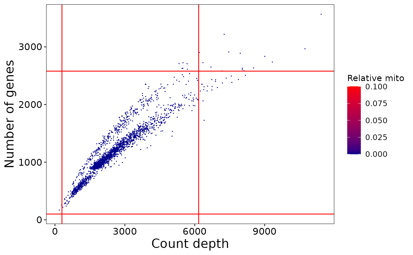
After running annotate_sce we may examine the plots and assess whether the applied thresholds are sensible for the sample. The effects of different parameters can be explored by iterating through the above generate_sce and annotate_sce functions until satisfied with the settings.
The next step is to filter the SingleCellExperiment with filter_sce: -
sce <- filter_sce(sce)
## ══ Filtering SingleCellExperiment ══════════════════════════════════════════════
## Pre-filtered SingleCellExperiment contains 15882 genes and 2188 cells.
## ✔ 60/0 mitochondrial genes were dropped.
## ✔ 0/79 ribosomal genes were dropped.
## ✔ 280/280 unmapped genes were dropped.
## ✔ 7390 non-expressive genes were dropped.
## ✔ 8309/15882 genes passed QC.
## ✔ 44 cells failed QC and were dropped: -
## Library size QC: PASS: 2186/FAIL: 2
## Number of genes QC: PASS: 2188/FAIL: 0
## Mitochondria counts proportion QC: PASS: 2188/FAIL: 0
## Ribosomal counts proportion QC: PASS: 2188/FAIL: 0
## Overall cell QC: PASS: 2144/FAIL: 44
## ✔ SingleCellExperiment was filtered successfully to 8309 genes and 2144 cells.
Step three – Finding singlets and discarding multiplets
At this stage we may wish to identify singlets in the SingleCellExperiment and discard any multiplets. In scFlow we simply run find_singlets and specify our preferred multiplet identification algorithm. Here we will use doubletfinder (This will take a while depending on the cell numbers):-
sce <- find_singlets(sce, "doubletfinder", pK = 0.005, vars_to_regress_out = c("nCount_RNA", "pc_mito"))Now we can filter out these multiplets with filter_sce:-
sce <- filter_sce(sce)You can see the remaining cells after all the filtering done by:
dim(sce)
## [1] 8309 2107
Finally we produce a report with report_qc_sce (this takes a few minutes): -
#Store results in same temp dir
report_qc_sce(sce, report_file = "qc_report_scflow_individual_1",
              report_folder_path = file.path(outputDir,"/tmp_Zeisel2015_scflow/"))
## ══ Generating QC report for SingleCellExperiment ═══════════════════════════════
## class: SingleCellExperiment
## dim: 8309 2107
## metadata(8): metadata scflow_steps ... citations doubletfinder_params
## assays(1): counts
## rownames(8309): ENSG00000000003 ENSG00000000419 ... ENSG00000285053
##   ENSG00000285441
## rowData names(13): ensembl_gene_id gene_biotype ...
##   qc_metric_is_expressive qc_metric_gene_passed
## colnames(2107): majos_Teinh_1 majos_Teinh_2 ... majos_MOL1_2187
##   majos_MOL1_2188
## colData names(18): barcode manifest ... qc_metric_max_features
##   is_singlet
## reducedDimNames(3): pca_by_individual tsne_by_individual
##   umap_by_individual
## mainExpName: NULL
## altExpNames(0):
And save our SingleCellExperiment: -
#create dir to hold resulting sce
dir.create(file.path(outputDir,"/sce_individual_1"))
write_sce(sce, folder_path= file.path(outputDir,"/sce_individual_1"))
Step four – Merging multiple datasets into one SingleCellExperiment object
Follow step one-three for all individual samples and save them using write_sce function. Then we read the individual SingleCellExperiment using read_sce into a list and merge them using merge_sce function. Begin by reading in the manifest and samplesheet and listing the file path to all individuals:
manifest <- read.delim(manifest_fp)
samplesheet <- read.delim(samplesheet_fp)
dir_list <-
  dir(path = file.path(outputDir,"/tmp_Zeisel2015_scflow"),
        pattern = "individual_[0-9]$", full.names = TRUE)
dir_list
## [1] "/tmp/RtmpWmQoYJ//tmp_Zeisel2015_scflow/individual_1"
## [2] "/tmp/RtmpWmQoYJ//tmp_Zeisel2015_scflow/individual_2"
## [3] "/tmp/RtmpWmQoYJ//tmp_Zeisel2015_scflow/individual_3"
## [4] "/tmp/RtmpWmQoYJ//tmp_Zeisel2015_scflow/individual_4"
## [5] "/tmp/RtmpWmQoYJ//tmp_Zeisel2015_scflow/individual_5"
## [6] "/tmp/RtmpWmQoYJ//tmp_Zeisel2015_scflow/individual_6"
Now loop through each, performing the analysis and finally merging the results:
sce_list <- list()

for(i in dir_list){
  mat <- read_sparse_matrix(i)
  metadata <- read_metadata(
    unique_key = manifest$key[as.numeric(gsub("individual_", "", basename(i)))],
    key_colname = "manifest",
    samplesheet_path = samplesheet_fp
  )
  var_classes <- c(
    individual = "factor"
  )
  metadata <- read_metadata(
    unique_key = manifest$key[as.numeric(gsub("individual_", "", basename(i)))],
    key_colname = "manifest",
    samplesheet_path = samplesheet_fp,
    col_classes = var_classes
  )
  sce <- generate_sce(mat, metadata)
  sce <- annotate_sce(
    sce,
    ensembl_mapping_file = ensembl_fp
  )
  sce <- filter_sce(sce)
  sce <- find_singlets(sce, "doubletfinder", pK = 0.005,
                        vars_to_regress_out = c("nCount_RNA", "pc_mito"),
                        num.cores = 1)
  sce <- filter_sce(sce)
  outdir <- file.path(outputDir,"/scflow_vignette_data")
  dir.create(outdir, showWarnings = FALSE)

  dir_report <- file.path(outdir, "qc_report")
  dir.create(dir_report, showWarnings = FALSE)

  #report_qc_sce(sce, report_file = paste0("qc_report_", basename(i)),
  #              report_folder_path = dir_report)

  sce_list[[basename(i)]] <- sce

}

sce <- merge_sce(
  sce_list,
  ensembl_mapping_file = ensembl_fp
)
After merging individual sce objects we can annotate and get an interactive html report on the merged sce using annotate_merged_sce and report_merged_sce functions respectively. Then we write the merged SingleCellExperiment object.
final_sce <- file.path(outdir, "sce")
dir.create(final_sce)
#annotate and save sce
sce <- annotate_merged_sce(sce)
write_sce(sce = sce,
          folder_path = final_sce,
          overwrite = TRUE)
Step five – Dataset integration, dimension reduction and clustering
Once we merge all the samples into one SingleCellExperiment object we can move to the next steps of integration, dimension reduction and clustering. We have implemented liger for integrating datasets from multiple samples, treatment and experiments. For optimal integration user should try to use different k values.
Once data integration is done, dimension reduction is performed using multiple methods by default i.e. “PCA”, “tSNE”, “UMAP”, “UMAP3D”. For tSNE and UMAP, dimension reduction is performed using either PCA or Liger values. Once the dimension reduction step is done the SingleCellExperiment object is ready for clustering.
dim(sce)
## [1]  9902 12438
#sample genes and samples for speed
sce <- integrate_sce(sce, method = "Liger", k = 20)
sce <- reduce_dims_sce(sce, pca_dims = 5, reduction_methods = "UMAP")
We can now plot UMAP generated using liger valuses using the following command:-
plot_reduced_dim(sce, feature_dim = "diagnosis",
                 reduced_dim = "UMAP_Liger", alpha = 1, size = 1)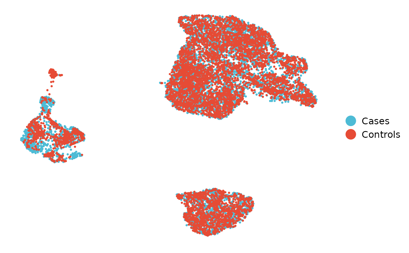
The next step is to cluster all the cells using cluster_sce command.
sce <- cluster_sce(sce, reduction_method = "UMAP_Liger", pca_dims = 5, k = 50,
                   resolution = NULL)
We can then plot the clusters:-
plot_reduced_dim(sce, feature_dim = "clusters",
                 reduced_dim = "UMAP_Liger", alpha = 1, size = 1)
The next step is to annotate the celltypes for each cluster. Here, we will use the package ewce. For this we use the following command (This may take a while). To know how the ctd was generated please visit EWCE package webpage. Users can generate and provide custom ctd. The annotation level can be an integer or a named list as shown in the code.
sce <- map_celltypes_sce(sce,
                         ctd_folder = ctd_fp,
                         annotation_level = list("ctd_AIBS_v2" = c(1,2)),
                         label_index = 1)
The celltypes for each cell can be found in sce@colData$cluster_celltype slot. We can also generate UMAP_Liger plot for each celltype.
plot_reduced_dim(sce,
                 feature_dim = "cluster_celltype",
                 reduced_dim = "UMAP_Liger",
                 alpha = 1,
                 size = 1)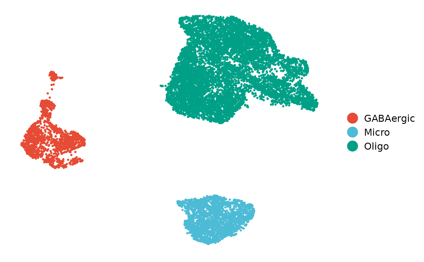
Our pipeline generates multiple reports. report_integrated_sce generates a report on integration whereas report_celltype_metrics generates detailed metrics on cell type distribution. Before running report_integrated_sce and report_celltype_metrics, the user needs to run annotate_integrated_sce and annotate_celltype_metrics functions respectively.
Step six – Performing differential expression analysis following by impacted pathway analysis
We need to subset the merged SingleCellExperiment object to perform differential expression analysis. Here we are using MASTZLM for differential expression analysis. For example, we are interested in performing DE analysis in the Oligo cell cluster. So, we first subset the Oligo cluster.
sce_subset <- sce[, sce$clusters == 1]We need to specify the colData column name as dependent_var as the variable of interest for DE analysis. For example here we want to perform DE analysis between Case and Controls which is found in diagnosis column. ref_class is the reference group for DE analysis. If there are any confounding variables those colData names can be passed through confounding_vars argument.
result_de <- perform_de(
  sce_subset,
  mast_method = "glmer",
  min_counts = 1,
  min_cells_pc = 0.25,
  dependent_var = "diagnosis",
  ref_class = "Controls",
  confounding_vars = c("cngeneson"),
  random_effects_var = "manifest",
  ensembl_mapping_file = ensembl_fp,
  nAGQ = 0)
result_de returns a list of DE tables based on how many contrast is being done in one celltype.
DT::datatable(result_de$diagnosisCases_vs_Controls,
              rownames = FALSE,
              escape = FALSE,
              options = list(pageLength = 5,
                             scrollX=T,
                             autoWidth = TRUE,
                             dom = 'Blfrtip'))
We have implemented two different functional enrichment tools enrichR and WebGestaltR. Users can call both tools using find_impacted_pathway() function. Here we will use enrichR only. A report can be generated on the output of the find_impacted_pathway() function using report_impacted_pathway().
# Get the significant genes for impacted pathway analysis

sig_de <- result_de$diagnosisCases_vs_Controls %>%
  dplyr::filter(padj <= 0.05, abs(logFC) >= 1.5) %>%
  dplyr::pull(gene) %>%
  as.character()

enrichment_result <- pathway_analysis_enrichr(
  sig_de,
  enrichment_database = c("GO_Biological_Process_2021",
"KEGG_2021_Human"))Step seven – Additional analysis
Single cell RNA seq data enables to study cell type composition in tissue and as a result we can perform a differential cell type composition analysis. We have implemented Dirichlet-multinomial regression analysis to compare cell type composition changes across a categorical dependent variables. model_celltype_freqs performs the differential composition analysis and generate plots. Here we will compare if there are any changes in the composition of cell types between Controls and Cases. Additional confounding variables can be passed via confounding_vars parameter.
results <- model_celltype_freqs(
  sce,
  unique_id_var = "manifest",
  celltype_var = "cluster_celltype",
  dependent_var = "diagnosis",
  ref_class = "Controls",
  var_order = c("Controls", "Cases")
)
``model_celltype_freq returns a list of plots and the pvalues from the analysis.
results$dirichlet_plot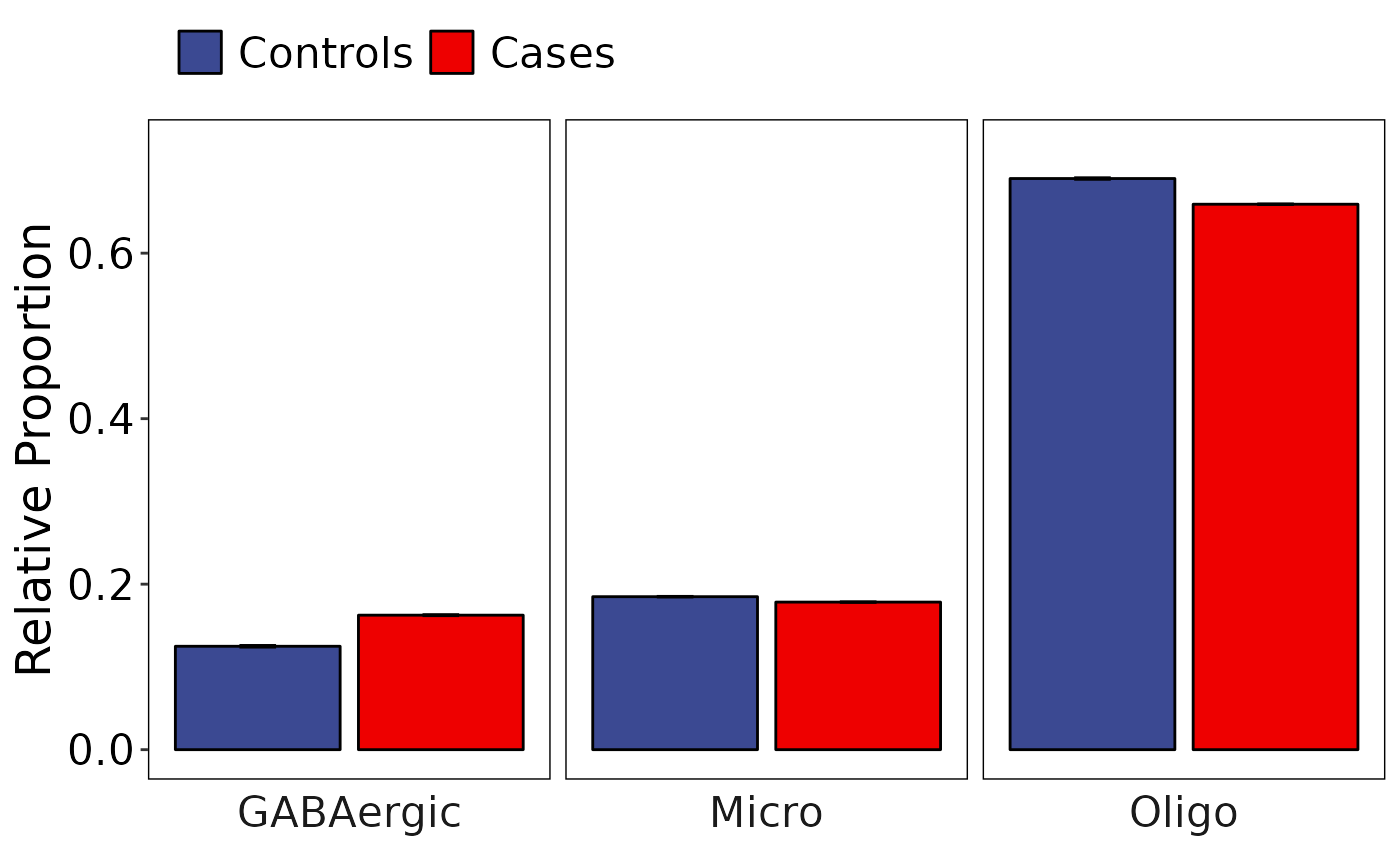
The complete result can be viewed as a html report generated by the function report_celltype_model.